Extrapolator_001
Download script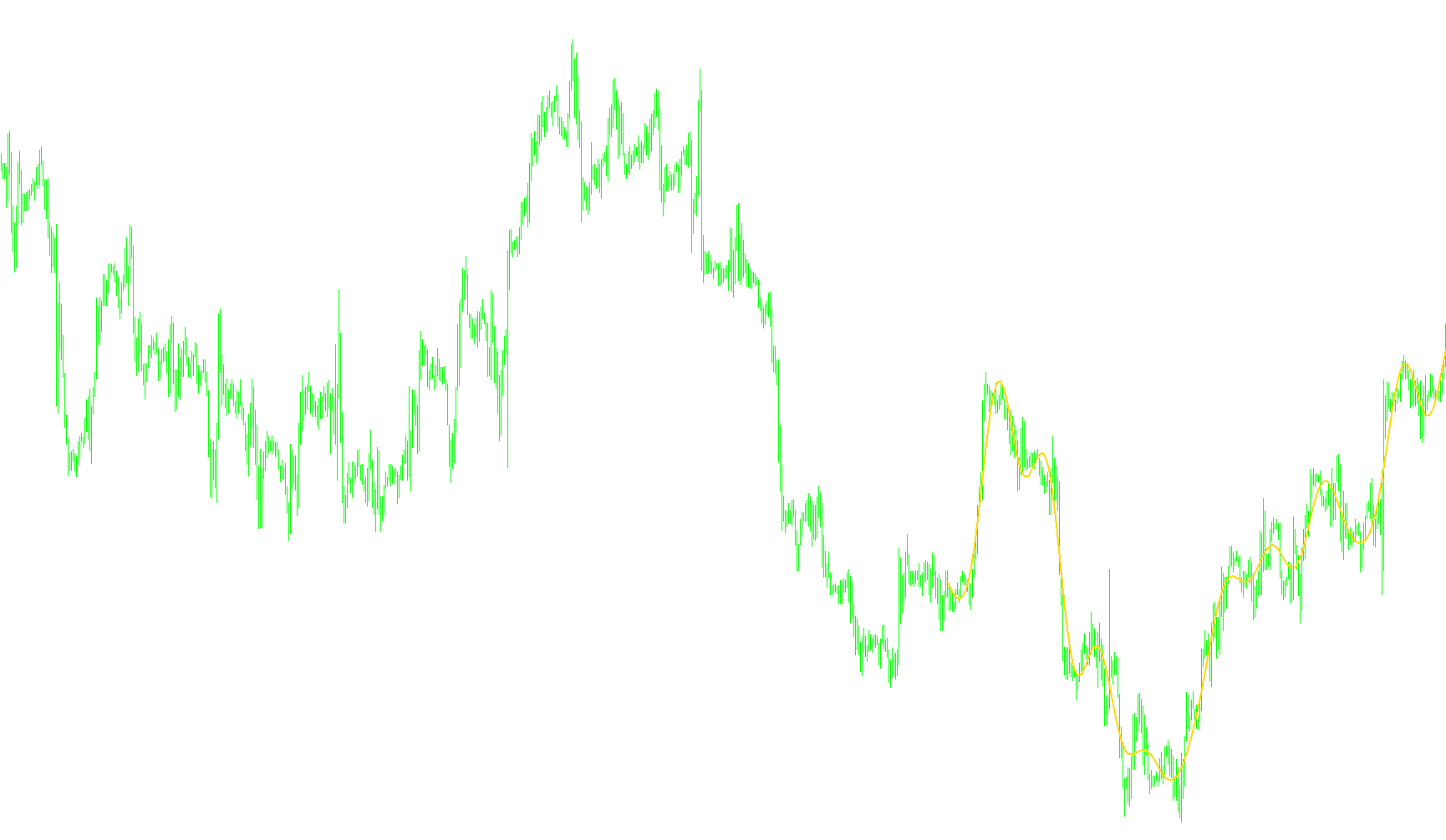
Overview of the Extrapolator Script
This script is a sophisticated mathematical tool designed to analyze historical price data and project potential future trends. In simple terms, it looks at "where the price has been" to calculate a logical path for "where the price might go next." Instead of just drawing a straight line from the last known point, it uses several complex engineering and statistical methods to identify patterns like cycles, waves, and momentum.
How It Works
The logic follows a three-step process: Data Preparation, Pattern Recognition, and Projection.
1. Data Preparation
The script begins by examining a specific window of past price data (which you can define in the settings). It calculates the average value of these prices to establish a "baseline." By subtracting this average from the actual prices, the script strips away the background noise, allowing it to focus purely on the fluctuations and trends of the market.
2. Pattern Recognition (The "Methods")
The core of the script is its ability to choose between different mathematical models to interpret these fluctuations. Users can select from six distinct methods:
- Trigonometric Fitting: This looks for repeating cycles (like waves). It attempts to find the frequency and "rhythm" of price movements to project them forward.
- Linear Prediction Models: These are several advanced statistical techniques (such as Autocorrelation, Burg, or Covariance methods) that treat the market like a complex signal. They calculate "coefficients"—basically weights—that determine how much the previous price movements influence the next one.
- Weighted and Geometric Methods: These provide even more granular analysis by giving more importance to recent data points than older ones, helping the prediction stay relevant to current market conditions.
3. Projection (Extrapolation)
Once the script has identified the underlying pattern (whether it is a wave, a specific trend, or a complex signal), it applies those rules to "future" bars on the chart. It generates a predicted path that extends beyond the current live price.
Key User Controls
To make the tool adjustable for different markets, it includes several customizable parameters:
- Method Selection: Allows you to switch between the six different mathematical logics mentioned above.
- Past/Future Bars: You can define how much history the script should "read" to make its calculation and how far into the future you want it to project the prediction.
- Prediction Order: This controls the complexity of the model; a higher order allows for more complex patterns but may become less stable, while a lower order is smoother.
- Frequency Tolerance: Specifically for the trigonometric method, this helps fine-tune how accurately the script detects cycles.
Summary
Think of this script as a "trend forecaster." While it cannot predict the future with certainty, it uses professional-grade signal processing and statistical modeling to visualize the most likely path the market will take based on the mathematical patterns found in its history.
//+--------------------------------------------------------------------------------------+
//|                                                                     Extrapolator.mq4 |
//|                                                               Copyright © 2008, gpwr |
//|                                                                   vlad1004@yahoo.com |
//+--------------------------------------------------------------------------------------+
#property copyright "Copyright © 2008, gpwr"
#property indicator_chart_window
#property indicator_buffers 2
#property indicator_color1 Blue
#property indicator_color2 Red
#property indicator_width1 2
#property indicator_width2 2

//Global constants
#define pi 3.141592653589793238462643383279502884197169399375105820974944592
/*
Method 1: Quinn-Fernandes Algorithm
Method 2: Autocorrelation Method
Method 3: Weighted Burg Method
Method 4: Burg Method with Helme-Nikias weighting function
Method 5: Itakura-Saito (geometric) method
Method 6: Modified covariance method
*/
//Input parameters
extern int     Method   =1;     //Extrapolation method
extern int     LastBar  =0;    //Last bar in the past data
extern int     PastBars =300;   //Number of past bars
extern double  LPOrder  =0.6;   //Order of linear prediction model; 0 to 1
//LPOrder*PastBars specifies the number of prediction coefficients a[1..LPOrder*PastBars] where a[0]=1
extern int     FutBars  =100;   //Number of bars to predict; for LP is set at PastBars-Order-1
extern int     HarmNo   =20;    //Number of frequencies for Mathod 1; HarmNo=0 computes PastBars harmonics
extern double  FreqTOL  =0.0001;//Tolerance of frequency calculation for Method 1
//FreqTOL > 0.001 may not converge
extern int     BurgWin  =0;     //Windowing function for Weighted Burg Method; 0=no window 1=Hamming 2=Parabolic

//Indicator buffers
double pv[];
double fv[];

//Global variables
double ETA,INFTY,SMNO;
int np,nf,lb,no,it;

int init()
{
   lb=LastBar;
   np=PastBars;
   no=LPOrder*PastBars;
   nf=FutBars;
   if(Method>1) nf=np-no-1;
   if(HarmNo==0) HarmNo=np;

   IndicatorBuffers(4);
   SetIndexBuffer(0,pv);
   SetIndexBuffer(1,fv);
   SetIndexStyle(0,DRAW_LINE,STYLE_SOLID,2);
   SetIndexStyle(1,DRAW_LINE,STYLE_SOLID,2);
   SetIndexShift(0,-lb);//past data vector 0..np-1; 0 corresponds to bar=lb
   SetIndexShift(1,nf-lb);//future data vector i=0..nf; nf corresponds to bar=lb
   IndicatorShortName("Extrapolator");
   return(0);
}

int deinit(){return(0);}

int start()
{
   ArrayInitialize(pv,EMPTY_VALUE);
   ArrayInitialize(fv,EMPTY_VALUE);

//Find average of past values
   double av=0.0;
   for(int i=0;i<np;i++) av+=Open[i+lb];
   av/=np;

//Prepare data
   if(Method==1)
   {
      for(i=0;i<np;i++)
      {
         pv[i]=av;
         if(i<=nf) fv[i]=av;
      }
   }
   else
   {
      double a[],x[];
      ArrayResize(a,no+1);
      ArrayResize(x,np);
      for(i=0;i<np;i++) x[np-1-i]=Open[i+lb]-av;
   }

//Select extrapolation method
   switch(Method)
   {
      case 1: //Fit trigomometric series
         double w,m,c,s;
         for(int harm=0;harm<HarmNo;harm++)
         {
            Freq(w,m,c,s);
            for(i=0;i<np;i++)
            {
               pv[i]+=m+c*MathCos(w*i)+s*MathSin(w*i);
               if(i<=nf) fv[i]+=m+c*MathCos(w*i)-s*MathSin(w*i);
            }
         }
         break;
      //Use linear prediction
      case 2: ACF(x,no,a);break;
      case 3: WBurg(x,no,BurgWin,a);break;
      case 4: HNBurg(x,no,a);break;
      case 5: Geom(x,no,a);break;
      case 6:
         bool stop=0;
         MCov(x,no,a,stop);
         if(stop==1)
         {
            Print("Terminated prematurely");
            return(0);
         }
         for(i=no;i>=1;i--) a[i]=a[i-1];
   }

//Calculate linear predictions
   if(Method>1)
   {
      for(int n=no;n<np+nf;n++)
      {
         double sum=0.0;
         for(i=1;i<=no;i++)
            if(n-i<np) sum-=a[i]*x[n-i];
            else sum-=a[i]*fv[n-i-np+1];
         if(n<np) pv[np-1-n]=sum;
         else fv[n-np+1]=sum;
      }
      fv[0]=pv[0];

      for(i=0;i<np-no;i++)
      {
         pv[i]+=av;
         fv[i]+=av;
      }
   }

//Reorder the predicted vector
   for(i=0;i<=(nf-1)/2;i++)
   {
      double tmp=fv[i];
      fv[i]=fv[nf-i];
      fv[nf-i]=tmp;
   }
   return(0);
}
//+--------------------------------------------------------------------------------------+
//Quinn and Fernandes algorithm
void Freq(double& w, double& m, double& c, double& s)
{
   double z[],num,den;
   ArrayResize(z,np);
   double a=0.0;
   double b=2.0;
   z[0]=Open[lb]-pv[0];
   while(MathAbs(a-b)>FreqTOL)
   {
      a=b;
      z[1]=Open[1+lb]-pv[1]+a*z[0];
      num=z[0]*z[1];
      den=z[0]*z[0];
      for(int i=2;i<np;i++)
      {
         z[i]=Open[i+lb]-pv[i]+a*z[i-1]-z[i-2];
         num+=z[i-1]*(z[i]+z[i-2]);
         den+=z[i-1]*z[i-1];
      }
      b=num/den;
   }
   w=MathArccos(b/2.0);
   Fit(w,m,c,s);
   return;
}
//+-------------------------------------------------------------------------+
void Fit(double w, double& m, double& c, double& s)
{
   double Sc=0.0;
   double Ss=0.0;
   double Scc=0.0;
   double Sss=0.0;
   double Scs=0.0;
   double Sx=0.0;
   double Sxx=0.0;
   double Sxc=0.0;
   double Sxs=0.0;
   for(int i=0;i<np;i++)
   {
      double cos=MathCos(w*i);
      double sin=MathSin(w*i);
      Sc+=cos;
      Ss+=sin;
      Scc+=cos*cos;
      Sss+=sin*sin;
      Scs+=cos*sin;
      Sx+=(Open[i+lb]-pv[i]);
      Sxx+=MathPow(Open[i+lb]-pv[i],2);
      Sxc+=(Open[i+lb]-pv[i])*cos;
      Sxs+=(Open[i+lb]-pv[i])*sin;
   }
   Sc/=np;
   Ss/=np;
   Scc/=np;
   Sss/=np;
   Scs/=np;
   Sx/=np;
   Sxx/=np;
   Sxc/=np;
   Sxs/=np;
   if(w==0.0)
   {
      m=Sx;
      c=0.0;
      s=0.0;
   }
   else
   {
      //calculating c, s, and m
      double den=MathPow(Scs-Sc*Ss,2)-(Scc-Sc*Sc)*(Sss-Ss*Ss);
      c=((Sxs-Sx*Ss)*(Scs-Sc*Ss)-(Sxc-Sx*Sc)*(Sss-Ss*Ss))/den;
      s=((Sxc-Sx*Sc)*(Scs-Sc*Ss)-(Sxs-Sx*Ss)*(Scc-Sc*Sc))/den;
      m=Sx-c*Sc-s*Ss;
   }
   return;
}
//+-------------------------------------------------------------------------+
void ACF(double x[], int p, double& a[])
{
   int n=ArraySize(x);
   double rxx[],r,E,tmp;
   ArrayResize(rxx,p+1);
   int i,j,k,kh,ki;
   //Initialize
   for(j=0;j<=p;j++)
   {
      rxx[j]=0.0;
      for(i=j;i<n;i++) rxx[j]+=x[i]*x[i-j];
   }
   E=rxx[0];
   //Main loop
   for(k=1;k<=p;k++)
   {
      //Calculate reflection coefficient
      r=-rxx[k];
      for(i=1;i<k;i++) r-=a[i]*rxx[k-i];
      r/=E;
      //Calculate prediction coefficients
      a[k]=r;
      kh=k/2;
      for(i=1;i<=kh;i++)
	   {
	     ki=k-i;
	     tmp=a[i];
	     a[i]+=r*a[ki];
	     if(i!=ki) a[ki]+=r*tmp;
	   }
	   //Calculate new residual energy
      E*=(1-r*r);
   }
}
//+-------------------------------------------------------------------------+
void WBurg(double x[], int p, int w, double& a[])
{
   int n=ArraySize(x);
   double df[],db[];
   ArrayResize(df,n);
   ArrayResize(db,n);
   int i,k,kh,ki;
   double tmp,num,den,r;
   for(i=0;i<n;i++)
   {
      df[i]=x[i];
      db[i]=x[i];
   }
   //Main loop
   for(k=1;k<=p;k++)
   {
      //Calculate reflection coefficient
      num=0.0;
      den=0.0;
      if(k==1)
      {
         for(i=2;i<n;i++)
         {
            num+=win(i,2,n,w)*x[i-1]*(x[i]+x[i-2]);
            den+=win(i,2,n,w)*x[i-1]*x[i-1];
         }
         r=-num/den/2.0;
         if(r>1) r=1.0;
         if(r<-1.0) r=-1.0;
      }
      else
      {
         for(i=k;i<n;i++)
         {
            num+=win(i,k,n,w)*df[i]*db[i-1];
            den+=win(i,k,n,w)*(df[i]*df[i]+db[i-1]*db[i-1]);
         }
         r=-2.0*num/den;
      }
      //Calculate prediction coefficients
      a[k]=r;
      kh=k/2;
      for(i=1;i<=kh;i++)
	   {
	     ki=k-i;
	     tmp=a[i];
	     a[i]+=r*a[ki];
	     if(i!=ki) a[ki]+=r*tmp;
	   }
	   if(k<p)
         //Calculate new residues
         for(i=n-1;i>=k;i--)
         {
            tmp=df[i];
            df[i]+=r*db[i-1];
            db[i]=db[i-1]+r*tmp;
         }
   }
}
//+-------------------------------------------------------------------------+
double win(int i, int k, int n, int w)
{
   if(w==0) return(1.0);
   if(w==1) return(0.54-0.46*MathCos(pi*(2.0*(i-k)+1.0)/(n-k)));
   if(w==2) return(6.0*(i-k+1.0)*(n-i)/(n-k)/(n-k+1.0)/(n-k+2.0));
}
//+-------------------------------------------------------------------------+
void HNBurg(double x[], int p, double& a[])
{
   int n=ArraySize(x);
   double df[],db[];
   ArrayResize(df,n);
   ArrayResize(db,n);
   int i,k,kh,ki;
   double w,tmp,num,den,r;
   for(i=0;i<n;i++)
   {
      df[i]=x[i];
      db[i]=x[i];
   }
   //Main loop
   for(k=1;k<=p;k++)
   {
      //Calculate reflection coefficient
      num=0.0;
      den=0.0;
      if(k==1)
      {
         for(i=2;i<n;i++)
         {
            w=x[i-1]*x[i-1];
            num+=w*x[i-1]*(x[i]+x[i-2]);
            den+=w*x[i-1]*x[i-1];
         }
         r=-num/den/2.0;
         if(r>1) r=1.0;
         if(r<-1.0) r=-1.0;
      }
      else
      {
         w=0.0;
         for(i=1;i<k;i++) w+=x[i]*x[i];
         for(i=k;i<n;i++)
         {
            num+=w*df[i]*db[i-1];
            den+=w*(df[i]*df[i]+db[i-1]*db[i-1]);
            w=w+x[i]*x[i]-x[i-k+1]*x[i-k+1];
         }
         r=-2.0*num/den;
      }
      //Calculate prediction coefficients
      a[k]=r;
      kh=k/2;
      for(i=1;i<=kh;i++)
	   {
	     ki=k-i;
	     tmp=a[i];
	     a[i]+=r*a[ki];
	     if(i!=ki) a[ki]+=r*tmp;
	   }
	   if(k<p)
         //Calculate new residues
         for(i=n-1;i>=k;i--)
         {
            tmp=df[i];
            df[i]+=r*db[i-1];
            db[i]=db[i-1]+r*tmp;
         }
   }
}
//+-------------------------------------------------------------------------+
void Geom(double x[], int p, double& a[])
{
   int n=ArraySize(x);
   double df[],db[];
   ArrayResize(df,n);
   ArrayResize(db,n);
   int i,k,kh,ki;
   double tmp,num,denf,denb,r;
   for(i=0;i<n;i++)
   {
      df[i]=x[i];
      db[i]=x[i];
   }
   //Main loop
   for(k=1;k<=p;k++)
   {
      //Calculate reflection coefficient
      num=0.0;
      denf=0.0;
      denb=0.0;
      for(i=k;i<n;i++)
      {
         num+=df[i]*db[i-1];
         denf+=df[i]*df[i];
         denb+=db[i-1]*db[i-1];
      }
      r=-num/MathSqrt(denf)/MathSqrt(denb);
      //Calculate prediction coefficients
      a[k]=r;
      kh=k/2;
      for(i=1;i<=kh;i++)
	   {
	     ki=k-i;
	     tmp=a[i];
	     a[i]+=r*a[ki];
	     if(i!=ki) a[ki]+=r*tmp;
	   }
	   if(k<p)
         //Calculate new residues
         for(i=n-1;i>=k;i--)
         {
            tmp=df[i];
            df[i]+=r*db[i-1];
            db[i]=db[i-1]+r*tmp;
         }
   }
}
//+-------------------------------------------------------------------------+
/* Modified Covariance method from Marple's book. It solves
e[j]=y[j]+SUM(a[i]*y[j-i-1],i=0...m-1), j=0..n-1
for a[] by the least-squares minimization of e[j] in both directions of j.
The code substitues y[j] with x[n-1-j] because, in the provided data,
x[0] is the latest data point. */
void MCov(double x[], int ip, double& a[], bool& stop)
{
   //Initialization
   int n=ArraySize(x);
   double c[],d[],r[],v;
   ArrayResize(c,ip+1);
   ArrayResize(d,ip+1);
   ArrayResize(r,ip);
   int k,m,mk;
   double r1,r2,r3,r4,r5,delta,gamma,lambda,theta,psi,xi;
   double save1,save2,save3,save4,c1,c2,c3,c4,ef,eb;
   r1=0.0;
   for(k=1;k<n-1;k++) r1+=2.0*x[k]*x[k];
   r2=x[n-1]*x[n-1];
   r3=x[0]*x[0];
   r4=1.0/(r1+2.0*(r2+r3));
   v=r1+r2+r3;
   delta=1.0-r2*r4;
   gamma=1.0-r3*r4;
   lambda=x[0]*x[n-1]*r4;
   c[0]=x[0]*r4;
   d[0]=x[n-1]*r4;

   //Main loop
   for(m=0;;m++)
   {
      save1=0.0;
      for(k=m+1;k<n;k++) save1+=x[n-1-k]*x[n-k+m];
      save1*=2.0;
      r[m]=save1;
      theta=x[0]*d[0];
      psi=x[0]*c[0];
      xi=x[n-1]*d[0];
      if(m>0)
      {
         for(k=1;k<=m;k++)
         {
           theta+=x[k]*d[k];
           psi+=x[k]*c[k];
           xi+=x[n-1-k]*d[k];
           r[k-1]-=(x[m]*x[m-k]+x[n-1-m]*x[n-1-m+k]);
           save1+=r[k-1]*a[m-k];
         }
      }
      //order update of a[]
      c1=-save1/v;
      a[m]=c1;
      v*=(1.0-c1*c1);
      if(m>0)
      {
         for(k=0;k<(m+1)/2;k++)
         {
           mk=m-k-1;
           save1=a[k];
           a[k]=save1+c1*a[mk];
           if(k!=mk) a[mk]+=c1*save1;
         }
      }
      if(m==ip-1)
      {
         v*=(0.5/(n-1-m));
         break;
      }
      //time update of c[],d[],gamma,delta, and lambda
      r1=1.0/(delta*gamma-lambda*lambda);
      c1=(theta*lambda+psi*delta)*r1;
      c2=(psi*lambda+theta*gamma)*r1;
      c3=(xi*lambda+theta*delta)*r1;
      c4=(theta*lambda+xi*gamma)*r1;
      for(k=0;k<=m/2;k++)
      {
         mk=m-k;
         save1=c[k];
         save2=d[k];
         save3=c[mk];
         save4=d[mk];
         c[k]+=(c1*save3+c2*save4);
         d[k]+=(c3*save3+c4*save4);
         if(k!=mk)
         {
            c[mk]+=(c1*save1+c2*save2);
            d[mk]+=(c3*save1+c4*save2);
         }
      }
      r2=psi*psi;
      r3=theta*theta;
      r4=xi*xi;
      r5=gamma-(r2*delta+r3*gamma+2.0*psi*lambda*theta)*r1;
      r2=delta-(r3*delta+r4*gamma+2.*theta*lambda*xi)*r1;
      gamma=r5;
      delta=r2;
      lambda+=(c3*psi+c4*theta);
      if(v<=0.0)
      {
         Print("Error: negative or zero variance in MCov");
         stop=true;
         return;
      }
      if(delta<=0.0 || delta>1.0 || gamma<=0.0 || gamma>1.0)
      {
         Print("Error: delta and gamma are outside (0,1) in MCov");
         stop=true;
         return;
      }
      //time update of a[]; order updates of c[],d[],gamma,delta, and lambda
      r1=1.0/v;
      r2=1.0/(delta*gamma-lambda*lambda);
      ef=x[n-m-2];
      eb=x[m+1];
      for(k=0;k<=m;k++)
      {
         ef+=a[k]*x[n-1-m+k];
         eb+=a[k]*x[m-k];
      }
      c1=eb*r1;
      c2=ef*r1;
      c3=(eb*delta+ef*lambda)*r2;
      c4=(ef*gamma+eb*lambda)*r2;
      for(k=m;k>=0;k--)
      {
         save1=a[k];
         a[k]=save1+c3*c[k]+c4*d[k];
         c[k+1]=c[k]+c1*save1;
         d[k+1]=d[k]+c2*save1;
      }
      c[0]=c1;
      d[0]=c2;
      r3=eb*eb;
      r4=ef*ef;
      v-=(r3*delta+r4*gamma+2.0*ef*eb*lambda)*r2;
      delta-=r4*r1;
      gamma-=r3*r1;
      lambda+=ef*eb*r1;
      if(v<=0.0)
      {
         Print("Error: negative or zero variance in MCov");
         stop=true;
         return(0);
      }
      if(delta<=0.0 || delta>1.0 || gamma<=0.0 || gamma>1.0)
      {
         Print("Error: delta and gamma are outside (0,1) in MCov");
         stop=true;
         return(0);
      }
   }
   //for(m=ip;m>=1;m--) a[m]=a[m-1];
   //a[0]=1.0;
}
Comments